Optimal transport computation using linear programmming

This is an example of how one can solve OT using linear programming for small cases. The cost matrix is sampled from Uniform(0,1). Naturally, this won’t work well with large $n$, as it’s $O(n^3)$ – see Sinkhorn, etc.

n = 5
# Cost matrix sampled from uniform distribution
dat = np.random.uniform(0, 1, (n, n))
print(dat.shape)
p = [1]*n # source marginal
q = [1]*n # target marginal

c = dat.reshape(1, -1)
c = c[0]

sp1 = identity(n, dtype=np.int8)
sp1_arr = sp1.todense()
sp2 = identity(n, dtype=np.int8)
sp2_arr = sp2.todense()

a1 = np.kron(p, sp1_arr)
a2 = np.kron(sp2_arr, q)

d = p + q
A = np.vstack((a1, a2))
res = linprog(c, A_eq=A, b_eq=d, options={'disp': True})
x = res.x
x[np.abs(x) < 0.0001] = 0

x2 = x.reshape((n, n), order='F')
print(f"solution is:\n {x2}")

The output is:

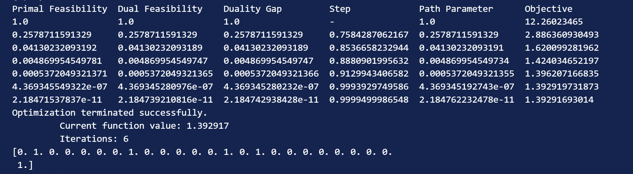
The reshaped vector is below, which tells us how the mass should move. For example, all the mass at 1 should be moved to 4.

[[0. 0. 0. 1. 0.] [1. 0. 0. 0. 0.] [0. 1. 0. 0. 0.] [0. 0. 1. 0. 0.] [0. 0. 0. 0. 1.]]